Summary of concepts involved in addressing our political and economic problems

This post summarizes some key ideas for a theoretical framework suitable for developing strategies for reversing American decline. I make no attempt to weave them into an overarching theory or to provide a program for American revival, such a synthesis is premature, even if it were possible.

Cultural evolution is the core mechanism through which history progresses
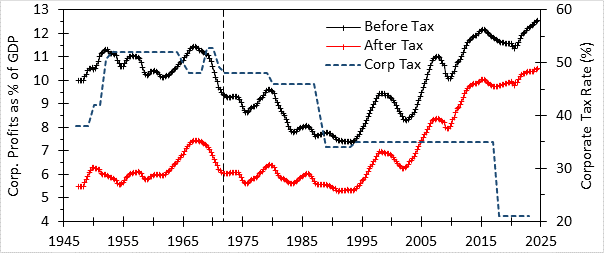
Economic theory and data indicate that higher tax rates depress economic growth. These studies employed statistical methods to estimate the impact of a change in tax rate on output or income. They indicate that higher taxes depressed growth rates and seem convincing to me. The results also makes sense from basic economic reasoning. If you tax something you get less of it, which has been shown by the effects of cigarette taxes on smoking rates. Given this, the excellent economic performance in the postwar era when income and corporate tax rates were much higher than today is puzzling. Paul Krugman notes that the postwar economy has been memory-holed because it is not consistent with these economic findings and with what supporters of low taxes on higher income individuals want to believe. In an effort to explain away this postwar anomaly economists have proposed “hand waving” explanations such as a lack of foreign competition from war-devasted economies. I address this and other arguments here.

The superior economic performance in the postwar era cannot be explained by economic theory. The tax structure then should have led to lower growth than what we have seen under the modern low-tax environment. Not explored in economic analysis like those I cited are effects over the longer term (decades) that cannot be addressed using natural experiments. Economists are aware of these things, which are usually called structural effects. Economic effects like the negative effect of taxes on growth apply within a given economic structure. The reason for the curious performance of the postwar economy is that the structure was different. During the high-tax postwar era structural effects produced strong growth as a basal condition, that was reduced by the deleterious economic effects of high taxes. The hand-waving arguments mentioned earlier are attempts to identify the structural factor responsible for the strong growth in order to explain why an economy like that is no longer possible, so we should just forget it ever happened.

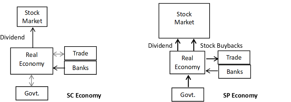
I have my own WAG that says the structural effects arise from cultural evolution. I posit there was a stakeholder capitalism (SC) economic culture operative in the postwar era and a shareholder primacy (SP) economic culture operative in the more recent economy. I presented the argument and some evidence for it in a peer-reviewed paper making it a SWAG. A shorter version of this argument is given here and here. I present a model whose output represents the relative amounts of SC and SP capitalism present over time (see “model” in this figure).

The core element of my SWAG is that capitalism is all about the accumulation of capital. Capital comes in two forms. One is real (productive) capital, defined as “the production factor that when combined with labor and resources leads to increased sales and profits.” The other is financial capital, defined as market capitalization. Under SC culture the objective of capitalist businessmen is growing real capital, resulting in economic growth in proportion to the capital accumulated. Under SP culture the objective is growing financial capital, economic growth happens as a side effect. Growing earnings and stock buybacks are the main ways SP capitalists achieve their objective function. Only the former leads to economic growth.

The economic effects still operate under both cultures. The profit level obtained under high-tax SC culture before 1980 was lower than it is under low tax SP culture. The higher profits generated under SP are largely used for stock buybacks and dividends rather than investment and do not contribute to economic growth. Investment that is made must compete with financial returns that are higher under SP capitalism. Investment is less productive, but more profitable, and the economy grows more slowly. I must stress that none of this is due to some moral shortfall among capitalists, as many frustrated with our modern economy appear to think based on the public reaction to the killing of a health insurance CEO. CEOs are people like everyone else and respond to the same incentives and cultural expectations as we all do. If you want better-behaved CEOs, then change the culture that provides the norms that regulate CEO behavior.

I have found a cultural evolutionary framework most useful for understanding structural economic changes, as it does not assume conspiracies, but just people being people. To paraphrase geneticist Theodosius G. Dobzhansky: nothing in human affairs makes sense except in light of (cultural) evolution.

Political Orders (dispensations) are important
Economic cultural evolution occurs in response to changes in the economic environment created by government-supplied economic policy. Policies arise out of politics, making politics and economics joined at the hip, a fact not lost on the founders of economics, who called their discipline political economy to reflect this fact.

To understand these political effects, I use Stephen Skowronek’s political time model, in which successive reconstructive presidents create political orders favoring their party that I call dispensations. Dispensations are important because they provide the ideologies that justify the economic policies that select for different economic cultures under cultural evolution. For example, Neoliberal policies, which select for SP capitalism, are the product of the Reagan dispensation. I oppose Neoliberalism and would like America to return to something like the New Deal Order, which would shift culture back to the SC culture prevalent in the postwar era. I describe myself as a New Dealer for that reason. I believe a new dispensation is necessary to enact the policy needed to make such a shift. My recent article on dispensations, outlined how several recent dispensations were instituted. I noted that the three most recent dispensation changes resulted from economic changes: for 1896, the onset of inflation, for 1932, strong wage growth, and for 1980 the end of high inflation.

Inflation is important
Two of the economic changes involved price inflation. A key factor in the evolution of the SC culture that maintained the FDR dispensation was the high tax rate policy enacted to deal with a perceived threat of inflation. Inflation has played a major role in recent dispensation changes and the associated political-economic culture shifts and may do so again. An overview of how inflation seems to work is instructive.

Evolution of thinking on inflation
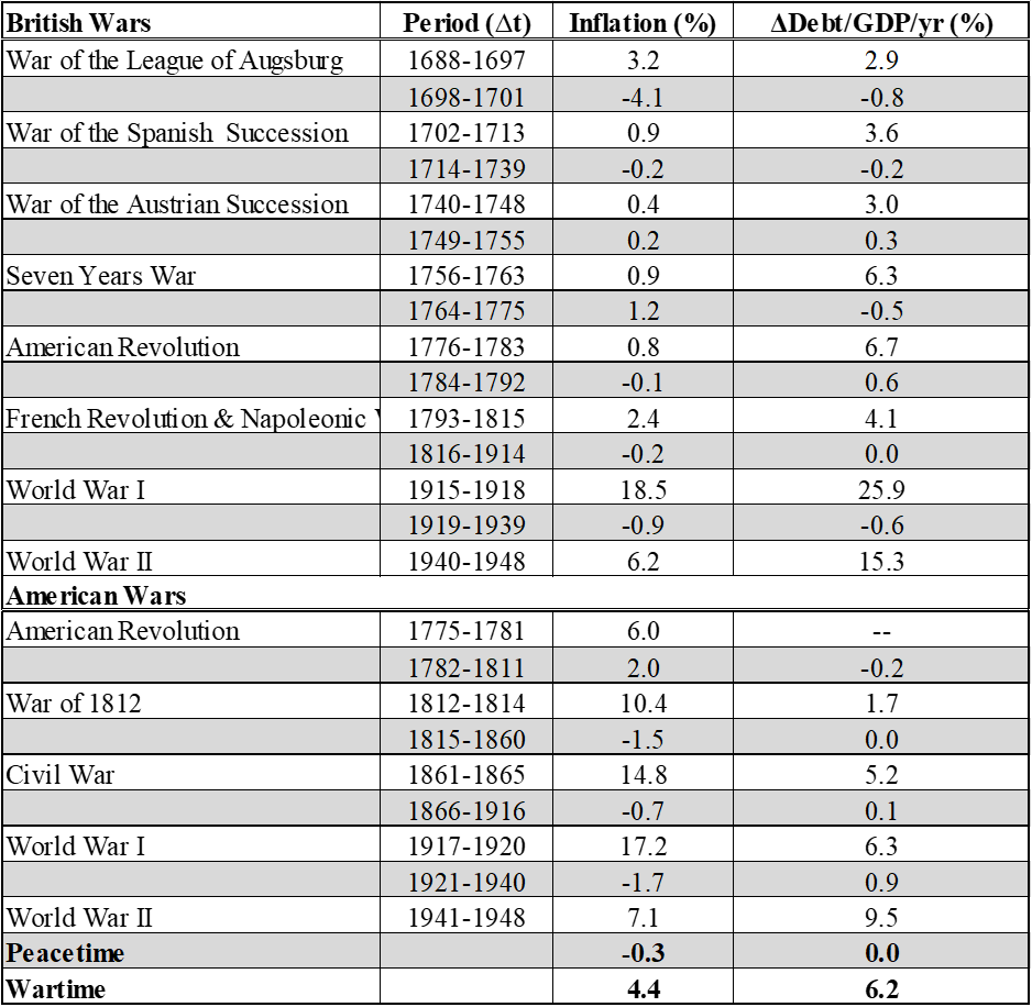
From the late 17th century through WW II, there was a relationship between inflation and government deficits that manifested during major wars in both Britain and America (see Table 1). Average inflation over 13 periods of wartime was 4.4% compared to -0.3% between the wars. Growth in government debt during wartime averaged 6.2%/yr compared to no growth during peacetime. This experience fostered a belief that deficits lead to inflation.

Table 1. Inflation and debt growth during war and peace

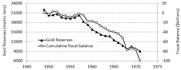
After WW II, efforts were made to maintain balanced budgets under both Presidents Truman and Eisenhower. These served to maintain the national gold reserve, which played an important role in economic management under the Bretton Woods system. In the 1960 election the issue of maintenance of this reserve came up. Nixon believed that maintaining the reserve was important in order to prevent inflation, Kennedy did not. Kennedy won, the gold reserve was allowed to decline and the Bretton Woods gold standard system collapsed in 1971. Nixon was president at this time but had changed his tune from 1960. He claimed he was now a Keynesian, adopted price controls after ending the gold standard, and continued to run deficits. The result was ruinous inflation when controls were lifted in Jan 1973 after Nixon was safely reelected. This began a decade of stagflation, a combination of inflation and high unemployment resulting from the high interest rates the Fed was using to combat inflation. Stagflation killed the FDR dispensation which gave conservatives the opportunity to enact Neoliberalism after Reagan’s victory in 1980. From this has come economic inequality, elite proliferation and political polarization, declining marriage rates, and, possibly, low fertility.

Since 1980, Republican policymakers have been unconcerned with deficits, as asserted by Vice President Dick Cheney: “Reagan proved deficits don’t matter.” Democrats continued to care about deficits through the 1990’s, when a budget surplus was achieved under President Clinton, but have since come to see the issue as the Republicans do.

Modeling inflation
Growing up during inflationary times, I had become a fiscal conservative by age 19. In the late 1990’s I was learning about investing and had developed an interest in economic cycles. I developed a simple valuation concept to find cycles in the stock market. My Stock Cycle was a subcycle of the longer Kondratiev cycle in price inflation. I wrote books about both. To characterize the Kondratiev cycle for the modern era in which price cycles no longer occurred, I developed an analysis based on the quantity theory of money:

1. PY = MV

Here P is the price level, Y is real output (i.e. real GDP), M is money supply and V is the velocity of circulation. MV is then the rate at which money changes hands over a year, and PY is the market value of net economic activity during that year. The idea behind equation 1 is that for a constant value of V, increases in M greater than increases in Y will result in higher prices (inflation). I have presented my original analysis elsewhere. Here I present a somewhat different (and more rigorous) approach.

The PY term on the left-hand side of equation 1 is just nominal GDP (i.e. with no inflation adjustment). M is some measure of money supply. Based on the pattern shown in Table 1, deficit spending (changes in government debt) appears to act like an increase in M in equation 1. In addition to this is the money creation resulting from lending by banks and other financial institutions. This kind of money is captured by various money supply measures. I chose M3 as the most comprehensive measure. Thus, M in my analysis is the sum of M3 and cumulative deficits, or government debt held by the public. With his I can write equation 1 as:

2. GDP = V (M3 + Debt)

My analysis back in 1999 used real GDP and the CPI for P. Much later, I realized that this approach had an inflation estimate (the GDP deflator used to calculate real GDP) buried in it and so it was unclear what I was measuring. For this analysis I decided to employ nominal GDP. This makes the three data sets used (GDP, M3 and deficit spending) all independent of each other, ensuring I am not measuring an artifact.

I added deficits since 1900 to the national debt in 1900) to give Debt for the years after 1900. I then regressed GDP against the sum of M3 and cumulative deficits/debt, fixing the intercept at a value that made the two sides of equation 2 equal for 1900. Thus, I was fitting only a single parameter, the average value of V over the interval considered. I found that the fit using the full 1900-2023 annual dataset was not that good. The fit I obtained using a 1900-1995 interval was much better (r² = 0.995). Figure 1 plots GDP and the regression equation over time. The closeness of the fit up to around 2000 is evident. I also plotted the ratio of the two, which may be thought of current velocity relative to its long-term average value.

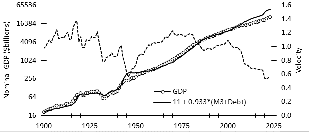
Figure 1. GDP and monetary model over 1900-2023, showing the ratio between the two

The value of this ratio spiked up for WW I (which traditionally is seen as a Kondratiev cycle peak). Following is a sharp drop from 1929 to 1933, reflecting the beginning of the great Depression, a peak in 1942, reflecting WW II, and a second strong drop to a trough in 1946, reflecting the impact of WW II price controls. The ratio rises from the 1946 trough to reach a broad top over 1970-81, reflecting the 1970’s stagflation. Next is a drop to a trough in 1986, due to Volcker’s war on inflation. A new rise follows with another peak around 2000 and a shallow drop to 2007, which is followed by strong drop in 2008, due to the financial crisis and second drop for the pandemic.

Rearranging equation 2 gives

3. V^-1 = (M3 + debt)/GDP = “amount of money chasing dollar-denominated output”

I then calculated the annual change in money (ΔM3 + Δdebt) divided by GDP for each year from 1900 to 2001. I had previously estimated NAIRU values for various periods between the end of WW II and the end of the century. Figure 2 presents the NAIRU value obtained for these periods plotted against the average value of Δmoney/ GDP over that period.

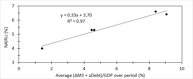
Figure 2. NAIRU versus average (ΔM3 + Δdebt)/GDP for the corresponding period

I got an excellent correlation between NAIRU and average Δmoney/ GDP, which I used to convert Δmoney/ GDP values into NAIRU values. NAIRU is the value of unemployment at which inflation is (theoretically) not supposed to change. If unemployment rises above NAIRU inflation falls, if it falls below, inflation rises. To test the utility of this idea I plotted NAIRU-Unemployment rate, a quantity I call the inflation driver, and CPI inflation over time in Figure 3. Figure 3 shows values of ID and inflation on monthly basis, data for which are only available back to 1960.

Figure 3. Inflation driver and inflation 1960-1995

Inflation driver (ID) is a qualitative indicator, it gives an inflationary signal when it rises above the dashed zero line and a deflationary signal when it falls below. The response to the inflationary signal appears to show a lag of about a year. For example, I note that ID began a sustained rise above zero in February 1964, but inflation did not begin an uptrend until 13 months later in March 1965. In contrast, the deflationary signal is fast acting: when ID fell below zero in February 1970, inflation started heading down the very next month.

When ID punched above the zero line in January 1971, inflation initially continued to fall, reflecting the lag. We would expect inflation to begin to rise around the beginning of 1972, but President Nixon had implemented price controls in late summer 1971 that lasted until the beginning of 1973 (see dashed lines in Figure 3). As a result, rising inflation was delayed until late 1972 and took off at the beginning of 1973 when controls were lifted. By this time ID was very high and did not fall below zero until September 1974. Two months later inflation peaked at 12.2% and then headed down.

ID went negative in Sept 1974, rose to touch zero in April 1976, and then then fell again before finally going strongly positive in June 1977. Inflation reached a minimum in December 1976, during this second dip, then rose to a slightly higher plateau, before heading strongly upward in April 1978, ten months after the inflationary signal from ID the previous June. Inflation rose steadily, reaching north of 12% in October 1979 when President Carter appointed Paul Volcker as Fed chief and the war on inflation began. ID went below zero in January 1980, and inflation started down in March. The war ended when ID moved above zero in August 1986 and inflation started rising five months later. ID remained largely positive until September 1990 when it moved strongly into negative territory. Inflation peaked the next month and then headed down.

The model begins to break down after 1990. About two years ago, I made a preliminary attempt to expand the scope of quantity analysis by defining an effective money supply as the net accumulation of money in the real economy after adjusting for flows “out” of the economy due to trade deficits and money flowing out of the economy and into the stock market through dividends and stock buybacks. My first Substack post was about this. Since then, I have collected better, more complete data and when I redid this analysis more rigorously, I found that addition of most of these extra money flows gave worse results than the approach described above. The only exception was including a flow out of the economy due to stock buybacks. When I subtract buybacks from deficits and M3 growth for the money term in equation 2, I got a good fit to GDP for the whole 1900-2023 period as shown here. Emboldened by this finding I used the quantity (ΔM3+Δdebt-buybacks)/GDP for the x value in Figure 2 to calculate NAIRU for use in inflation driver for the post-1995 period.

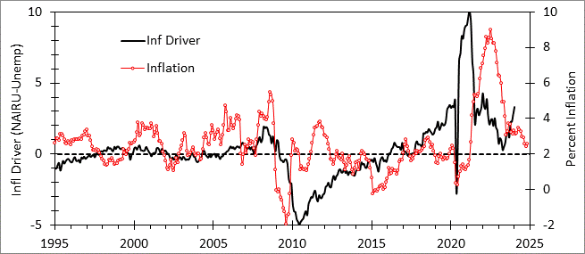
Figure 4. Inflation driver including stock buyback effect and inflation 1990-2025

The inflation driver with the buyback adjustment is plotted in Figure 4 for the period after 1995. We see the rising ID following the 1990 recession crossing the zero line at the beginning of 1998. Inflation begins moving higher fifteen months later in March 1999. It does not move decidedly below zero until March 2002, but inflation had peaked more than a year earlier, in January 2001, meaning the deflationary signal did not work like it had before. ID moved above zero in mid 2005, but inflation had entered an upward trend three years earlier, showing no connection. ID did begin a more rapid climb in 2008, which paralleled a rise in inflation, but again the drop below zero in February 2009 happened after inflation began its nosedive from August 2008 to August 2009. The signals provided by ID no longer matched up with the trend changes in inflation. Addition of the buyback adjustment extended the utility of this analysis by only a few years to the end of the 1990’s.

As we move closer to the present the correlation gets worse. ID shows a strong inflationary signal in 2016, with no corresponding inflationary response. The extremely strong spike in ID associated with the pandemic was followed a year and a half later by the large post-pandemic inflation spike, but ID never went below zero after that, completely missing the decline in inflation beginning in 2022. Although the trend in ID did shift strongly downward its failure to cross zero would lead one to support the idea that high inflation was going to remain a problem going forward, which did not happen. It appears that Cheney may have been on to something.

Things seem different today
It would seem that the stock market anomaly that gave rise to what may be a new stock market paradigm, has been joined by a change in the way the monetary system works. Gone are the days when deficits mattered in the simple direct way depicted in Figure 3 and the Fed controlled inflation by adjusting unemployment rate via interest rate adjustments. Interest rates still work to suppress inflation, has we have seen recently, but without significantly affecting unemployment (and hence the inflation driver). Presumably, downward adjustments of NAIRU, still work to reduce inflation as it certainly did after WW II (see Figure 5). I suspect faith in this relationship is behind calls for reductions in budget deficits.

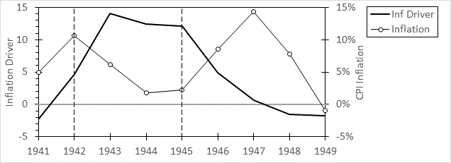
Figure 5. ID and inflation in during WW II and its aftermath

Figure 5 shows an ID analysis for the 1940’s, which is based on annual data, since monthly data before 1960 are not available. It shows a rapid rise in ID due to the Lend-Lease program that was reducing unemployment. With it came inflation. Price controls were implemented, which brought inflation down despite high ID. When they were lifted, ID was still strongly positive and inflation soared. But it was soon brought under control without massive interest rate hikes or higher unemployment (unemployment ran below 4% over 1946-48). A collapsing deficit produced a strong reduction in NAIRU, resulting in a declining ID without a rise in unemployment. ID crossed zero in 1947 after which inflation plummeted. This shows a New Deal economic policy that was missing in action during the 1960’s.

Summary and Conclusions
We have seen the three planks upon which rests a strong economy for all of us, not only elites. The first is cultural. Such an economy must feature something like stakeholder capitalism culture, in which the objective of capitalism is growth of the means of production—not just the values of investment assets such as stocks, real estate or crypto, as is the case under our present shareholder primacy culture. Business culture is set from the top down, by the CEO within a business and by economic policymakers for the economy as a whole. Policy is affected by the current elite-accepted economic ideology, and that is established by the current dispensation. The present Neoliberal Order is a product of the Reagan dispensation and is responsible for shareholder primacy culture. We cannot have one without the other. Changing the culture, requires changing the dispensation. Doing this has frequently involved dealing with inflation.

I developed a model and prediction tool for inflation that worked fairly well for the period from WW II to the end of the twentieth century. It provides support for my political stance as a fiscal conservative over 1978-2002. After then I threw in towel on balanced budgets, since Republican administrations would undo any progress made on the deficit. The analysis here supports my decision and also shows that my instincts about the desirability of balanced budgets in my youth were valid. Had 1960’s Democrats paid the same level of attention to balancing the budget as did 1990’s Democrats, we could be living in a much better world.

A final thought is the curious coincidence between the onset of extreme stock market valuations, the midpoint in the rise of shareholder primacy, and the end of money flows playing a major role in inflation, which all happened in the mid to late 1990’s. Sometime around then we had this massive paradigm shift in which all that matters is the vibes. Stock valuations are for your grandparents and deficits no longer matter. Market valuations are taken as meaningful measures. Elon Musk is the richest man in the world largely because of the $700,000 per car value assigned to his car company (for comparison, GM is valued at a more reasonable $20,000 per car). If his cars were valued the same as everyone else’s, nobody would care what he thought. How does one account for this 35-fold difference? It’s the vibes, man. In a world in which a Bitcoin lacking any tangible value can sell for $100K, is $700K for a car with the right vibes out of line? Who knows?

It is possible this new “vibes economy” plays a role in our seemingly inflation-resistant economy. By the analytical framework in Figure 3, today’s inflation driver is larger than any since WW II, including those that generated the 1970’s stagflation. It was this discrepancy between massive money creation and low inflation in the last decade that led me to the idea that flows of dollars out of the economy due to trade flows and increased financial flows might explain this inflation resistance, but I could not get the numbers to work out when I took a more rigorous look. Perhaps I am missing something. Good ideas are welcome in the comments.